Modeling
In the previous blog, we discussed design approaches, fundamental conventions and constructions, and modules, to lay the groundwork for Verilog design. This blog will introduce you to the modelling of actual hardware circuits in Verilog. So let’s start the blog with our first modeling.
Gate-level Modeling
The majority of digital design is now done at the gate or higher levels of abstraction. The circuit is expressed in terms of gates at the gate level (e.g., and, nand).
There is a one-to-one relationship between the logic circuit diagram and the Verilog description, hardware creation at this level is obvious to a user with a basic understanding of digital logic design.
Gate types
Logic gates can be used to create a logic circuit. Basic logic gates are supported as predefined primitives in Verilog. These primitives are instantiated similarly to modules, but they are predefined in Verilog and do not need a module description.
Basic gates may be used to create any logic circuit. Basic gates are classified into two types: and/or gates and buf/not gates.
One gate terminal is an output, while the other terminals are inputs. A gate’s output is examined whenever one of its inputs changes.
And/or Gates
And/or gates have a single scalar output and a number of scalar inputs. The and/or gates that are accessible in Verilog are:
- AND
- OR
- XOR
- NAND
- NOR
- XNOR
Figure 1 depicts the equivalent logic symbols for these gates. We’ll look at gates with two inputs. The output terminal is symbolised by the letter “out”. The input terminals are designated by the letters “a” and “b”.
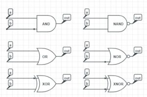
Fig1: Types of Gates
In Verilog, these gates are instantiated to form logic circuits. Some instances are shown below.
wire OUT, A,B;
//basic gate instantiations.
and a1(OUT,A,B);
or or1(OUT,A,B);
// 3 input gate
nand na1_3inp(OUT,A,B,C);
The truth table for these gates defines how the gategate’sputs are computed from their inputs. It is presumed that there are two input gates.
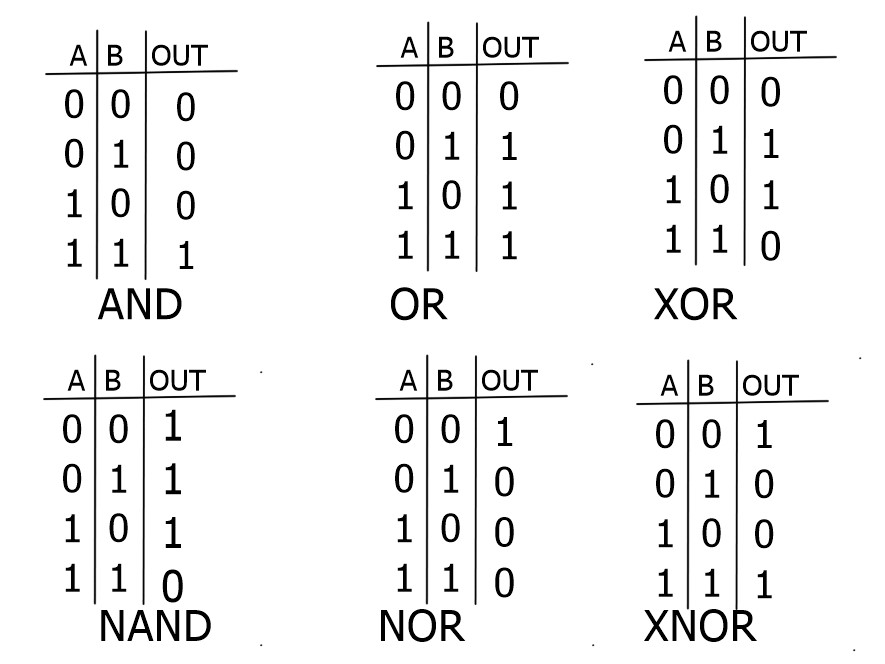
Fig2: Truth Table of Gates
Buf/Not Gates
Buf/not gates feature a single scalar input and several scalar outputs. The outputs are attached to the terminals at the end of the port list. We shall look at gates with only one input and one output. Verilog has two buf/not gate primitives are as follows:
- Buf
- NOT
Figure 3 depicts their symbols as well.
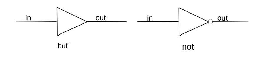
Fig 3: Buf and Not Gates
These gates, like them/or gates, are instantiated in Verilog. Their truth tables are much simpler because they have one input and the other end is an output.
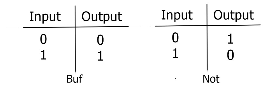
Fig 4: Buf and Not Gates Truth Table
Bufif/Notif Gates
Bufif and notif gates have extra control indications on the buf and not gates, respectively.
- Bufif1
- Bufif0
- Notif1
- Notif0
If this external control is asserted, then only the gate propagates and hence truth table is same as the buf and not gate.
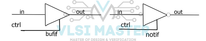
Fig 5: Butif and Notif symbols
And now we will move on to the next topic of our blog, i.e., dataflow modeling.
Dataflow Modeling
As previously discussed, the gate level modelling technique works extremely well since the number of gates is minimal and the designer may manually instantiate and link each gate.
However, as chip technology advances and gate densities on devices increase, dataflow modelling has become increasingly important. Logic synthesis is the process of creating a gate-level circuit from a dataflow design description using automated tools.
As logic synthesis tools have gotten more advanced, dataflow modelling has become a prominent design method. This method allows the designer to focus on improving the circuit’s data flow.
The RTL (register transfer level) design is widely used in the digital design field for a mix of data flow modelling and behavioural modelling.
Continuous Assignment
The most fundamental statement in dataflow modelling is a continuous assignment, which is used to drive a value into a net.
A continuous assignment substitutes gates in the circuit description and expresses them at a higher degree of abstraction. The term “assign” is used to begin a continuous assignment statement. An assign statement has the following syntax:
//simplest form of assign statement
 <continuous_assign> : := assign<drive_strength>?<delay>? <list_of_assignmenys>;
The following characteristics are shared by Continuous Assignment:
1. The assignment’s left side must always be a scalar or vector net, or a concatenation of scalar and vector nets.
2. Ongoing assignments are always in effect.
3. The right-hand operands might be registers, nets, or function calls.
4. Delay values in time units can be provided for assignments.
//continuous assign. out is a net. a and b are nets.
assign out = a & b;
Implicit Continuous Assignment
Instead of declaring a net and then writing a continuous assignment on it, Verilog provides a shortcut for placing a continuous assignment on a stated net. Because a net is only defined once, there might be implicit declaration assignment per net.
//regular continuous assignment
wire out;
assign out = a & b;
Delay
Delay values govern the period between when a right-hand operand changes and when the new value is allocated to the left-hand side.
Regular assignment delay, implicit continuous assignment delay, and net declaration delay are three techniques to define delays in continuous assignment statements.
When a delay is stated on a net, it can be defined without placing a continuous assignment on the net. Any value change made to a net out is postponed if a delay is specified on the net out. In gate-level modelling, net declaration delays can also be employed.
Expressions, operators, and Operands
Instead of primitive gates, dataflow modelling explains the architecture in terms of expressions. Dataflow modelling is built on expressions, operators, and operands.
Expressions
Expressions are mathematical constructions that combine operators and operands to yield a result.
Operands
Constants, integers, real numbers, nets, registers, times, bit-select, part-select, memory, or function calls can all be used as operands.
real a,b,c;
a=b+c; // b and c are real operands
Operators
Operators perform actions on operands to achieve the desired consequences. Verilog has a variety of operators.
a1 && a2 // && is an operator on operands a1 and a2
Operators
Operators can be arithmetic, logical, relational, equality, bitwise, reduction, shift, concatenation or conditional.
| Operator Types | Operator Symbol | Operation Formed | Number of Operands |
| Arithmetic | *
/ + – % |
Multiply
Divide Add Subtract modulus |
Two
Two Two Two Two |
| Logical | !
&& I I |
Logical negation
Logical and Logical or |
One
Two Two
|
| Relational | >
< >= <= |
Greater than
Less than Greater than or equal Lesser than or equal |
Two
Two Two Two |
| Equality | ~
& I ^ ^~ or ~^ |
Bitwise negation
Bitwise and Bitwise or Bitwise xor Bitwise xnor |
One
Two Two Two Two |
| Reduction | &
~& I ~I ^~ or ~^ |
Reduction and
Reductionn and Reduction or Reduction nor Reduction xnor
|
One
One One One One
|
| Shift | >>
<< |
Right Shift
Left Shift |
Two
Two |
| Concatenation
Replication |
{ }
{ {} } |
Concatenation
Replication |
Any number
Any number |
| Conditional | ?: | Conditonal | Three |
Table 1: Operators Types and Symbols
Behavioral Modeling
With the rising complexity of digital design, it is critical to make sound design decisions early in the project. Before deciding on the best architecture and algorithm to implement in hardware, designers must be able to analyse the trade-offs of alternative designs and algorithms.
The circuit is represented at a very high degree of abstraction in behavioural modelling. This level of design is more akin to C programming than to digital circuit design.
In many aspects, behavioural Verilog components are analogous to C language constructs. The Verilog is rich in behavioural constructs, which provide the designer a lot of leeway.
initial Statement
An initial block is made up of all statements that follow an initial statement. An initial block begins at time 0, executes precisely once throughout a simulation, and then stops.
If there are many beginning blocks, each one begins execution at time 0. Each block completes execution independently of the others.
Multiple behavioural assertions must be grouped together, usually using the keywords begin and stop. Grouping is not required if there is only one behavioural assertion. This is analogous to the begin-end blocks in Pascal programming or the groupings in C programming.
module stimulus;
reg x,y, a,b,m; initials
m=1'b0; // Single statement
always Statement
An always block is made up of all the behavioural assertions included within an always statement. The always statement begins at time 0 and loops through the statements in the always block indefinitely. This statement is used to represent a continuous block of activity in a digital circuit.
A clock generator module, for example, toggles the clock signal every half cycle. The clock generator in actual circuits is active from time 0 to as long as the circuit is switched on.
module clock_gen;
reg clock;
// at time zero
initials
    clock = 1'b0;
// at half ycle
always
    #10 clock = ~clock;
endmodule
Procedural Assignments
Procedural assignments change the values of variables such as reg, integer, real, and time. The value assigned to a variable remains unaltered until another procedural assignment replaces it with a different value.
Their syntax is very simple as shown below.
<assignment>
:: = <1value> = <expression>
There are two types of procedural assignments.
- Blocking assignments
Blocking assignments are carried out in the sequence stated in a sequential block.
- Nonblocking assignments
Nonblocking assignments allow assignments to be scheduled without interfering with the execution of the statements that follow in a sequential block.
Timing Controls
Verilog has a number of behavioural timing control mechanisms. If there are no timing control directives in Verilog, the simulation time does not advance.
Timing settings allow you to select the simulation time when procedural statements will be executed. Timing control may be accomplished in three ways: delay-based timing control, event-based timing control, and level-sensitive timing control.
Conditional Statement
Conditional statements are used to base judgments on certain criteria. These criteria are used to determine whether or not to execute a statement.
Loops
There are four types of loops that are used:
- While Loop
- For Loop
- Repeat Loop
- Forever Loop
So, let’s move to the last type of modelling.
Switch-level Modeling
Transistors are also known as switches that either conduct or are open in Verilog HDL. In this blog, we will go over the fundamentals of switch-level modelling.
Switch-Modeling Elements
Verilog has several constructs for modelling switch-level circuits. These components are used to characterise digital circuits at the MOS-transistor level.
MOS Switches
There are two types of MOS switches.
- NMOS
- PMOS
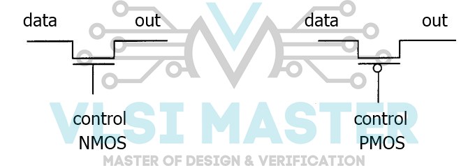
Fig 6: Switches
Instantiation of NMOS and PMOS are also simple as shown below.
pmos pl (out, data, control): //instantiate a pmos switch
nmos nl (out, data, control): //instantiate a nmos switch
CMOS Switches
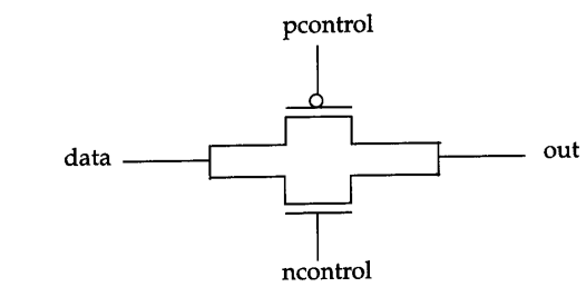
Fig 7: CMOS Switches
As shown in Figure 7, a cmos device can be constructed with an nmos and pmos device.
Bidirectional Switches
Gates such as NMOS, PMOS, and CMOS conduct from drain to source. It’s critical to have gadgets that can operate in both ways.
In such instances, the driving signal might come from either side of the device. For this reason, bidirectional switches are offered.
Power and Ground
When designing transistor-level circuits, power (Vdd, logic 1) and ground (Vss, logic 0) sources are required. The terms “supply1” and “supply0” are used to define power and ground sources.
supplyl vdd;
supply0 gnd;
assign a = vdd; //Connect a to vdd
assign b = gnd; //Connect b to gnd
Resistive Switches
MOS, CMOS, and bidirectional switches, as previously described, may be characterised as resistive devices.
Resistive switches have a larger source-to-drain impedance than conventional switches, lowering the signal power that passes through them. Resistive switches are denoted by keywords that are prefixed with an in comparison to the comparable keywords for ordinary switches.
The syntax of resistive switches is the same as that of ordinary switches.
rnmos rpmos // resistive nmos and pmos switches
So we finally read a long blog, but from it we must have understood all the basic things today related to different types of modelling.
Let us finally summarise what we have essentially studied.
- What are the four types of modeling?
- How many types of gates?
- How many types of dataflow modelling exist?
- What are the different types of operators?
- What are the types of statements used in behavioural modeling?
- Explain the various types of loops.
- What are the different types of switches in switch level modeling?